library(simplePHENOTYPES)
library(dplyr)
library(tibble)

data("SNP55K_maize282_maf04", package = "simplePHENOTYPES")
geno <- as_numeric(
  SNP55K_maize282_maf04,
  to_r = TRUE, to_file = FALSE, verbose = FALSE
)5 Additive phenotype models
The first chapter simulated one additive trait with default settings. This chapter opens the additive layer up: how the causal markers are chosen, how their effects are generated, how the layer is scaled to its requested share of the phenotypic variance, and what the per-marker var_explained diagnostic does and does not mean. It also shows the options of simulate_phenotype() that apply to every later chapter: replications, a phenotype mean, a subset of individuals, entry means, and the one-call form.
5.1 Worked example
5.1.1 Load the package and the maize genotypes
The data are the inbred maize panel used in A first simulation. The genotype-input chapter explains the format and its quality checks.
5.1.2 A single additive layer and its causal markers
simulate_phenotype() fixes the data, the seed, and the global settings; additive() adds one additive component. prop is the share of the phenotypic variance that the layer receives, and n_qtn is the number of causal markers, which the package calls QTNs (quantitative trait nucleotides).
sim <- simulate_phenotype(geno, seed = 11) |>
  additive(prop = 0.6, n_qtn = 10)
print(sim)
#> <phenotype_sim> (realized · long format)
#> Genotypes: geno Traits: 1 Architecture: independent Seed: 11
#> Variance partition (proportions of V_P):
#> additive 0.60 (10 QTNs, geometric)
#> residual 0.40
#> Requested genetic share = 0.60 realized H² = 0.61qt <- qtn_table(sim)
qt |>
select(snp, chr, pos, maf, effect, var_explained)| snp | chr | pos | maf | effect | var_explained |
|---|---|---|---|---|---|
| ss196490968 | 9 | 64724480 | 0.4857143 | 0.5000000 | 0.4355922 |
| ss196508164 | 6 | 152947840 | 0.4928571 | 0.2500000 | 0.1089653 |
| ss196524380 | 1 | 65659871 | 0.4821429 | 0.1250000 | 0.0274079 |
| ss196414723 | 1 | 242143315 | 0.4785714 | 0.0625000 | 0.0068481 |
| ss196448388 | 3 | 160083617 | 0.4446429 | 0.0312500 | 0.0016880 |
| ss196477747 | 7 | 83873489 | 0.4535714 | 0.0156250 | 0.0004251 |
| ss196466547 | 5 | 154351003 | 0.4160714 | 0.0078125 | 0.0001038 |
| ss196458769 | 4 | 195754416 | 0.4303571 | 0.0039063 | 0.0000262 |
| ss196497131 | 10 | 66872567 | 0.4214286 | 0.0019531 | 0.0000065 |
| ss196438181 | 2 | 130544751 | 0.4500000 | 0.0009766 | 0.0000017 |
qtn_table() lists the causal markers in the order they were drawn, together with the minor-allele frequency (maf), the effect assigned to each marker, and var_explained. The effects follow a geometric series: the first marker’s effect is 0.5, the second 0.25, and so on. The markers are a simple random sample of the markers that vary in the panel.
5.1.3 Effect series: geometric, custom base, or explicit effects
The effect argument changes the series. A single value is the base of the geometric series; a vector of length n_qtn is used as given. Equal effects give a trait where no single marker dominates.
base_09 <- simulate_phenotype(geno, seed = 11) |>
  additive(prop = 0.6, n_qtn = 10, effect = 0.9)

equal <- simulate_phenotype(geno, seed = 11) |>
  additive(prop = 0.6, n_qtn = 10, effect = rep(1, 10))

tibble(
  marker = seq_len(10),
  default = qtn_table(sim)$effect,
  base_0.9 = qtn_table(base_09)$effect,
  equal = qtn_table(equal)$effect
)| marker | default | base_0.9 | equal |
|---|---|---|---|
| 1 | 0.5000000 | 0.9000000 | 1 |
| 2 | 0.2500000 | 0.8100000 | 1 |
| 3 | 0.1250000 | 0.7290000 | 1 |
| 4 | 0.0625000 | 0.6561000 | 1 |
| 5 | 0.0312500 | 0.5904900 | 1 |
| 6 | 0.0156250 | 0.5314410 | 1 |
| 7 | 0.0078125 | 0.4782969 | 1 |
| 8 | 0.0039063 | 0.4304672 | 1 |
| 9 | 0.0019531 | 0.3874205 | 1 |
| 10 | 0.0009766 | 0.3486784 | 1 |
The three simulations share the same seed and therefore the same ten markers; only the effects differ. Because the layer is rescaled to prop afterwards, the absolute size of the effects does not matter. Only their relative sizes do. Multiplying every effect by the same constant leaves the phenotype unchanged.
phase = "repulsion" alternates the sign of successive effects in draw order. It is a bookkeeping convenience, not a phase read from the haplotypes: for unlinked markers it merely relabels which allele increases the trait. The multi-trait chapter shows the haplotype-derived phase of the "ld" architecture.
repulsion <- simulate_phenotype(geno, seed = 11) |>
  additive(prop = 0.6, n_qtn = 10, phase = "repulsion")

tibble(
  coupling = qtn_table(sim)$effect,
  repulsion = qtn_table(repulsion)$effect
)| coupling | repulsion |
|---|---|
| 0.5000000 | 0.5000000 |
| 0.2500000 | -0.2500000 |
| 0.1250000 | 0.1250000 |
| 0.0625000 | -0.0625000 |
| 0.0312500 | 0.0312500 |
| 0.0156250 | -0.0156250 |
| 0.0078125 | 0.0078125 |
| 0.0039063 | -0.0039063 |
| 0.0019531 | 0.0019531 |
| 0.0009766 | -0.0009766 |
5.1.4 Fix the causal markers yourself
qtn accepts marker names or column indices. This is the way to simulate a trait on loci chosen for a reason, for example genes from a known pathway or markers at a chosen allele frequency. n_qtn is then taken from the length of qtn.
chosen <- geno$snp[c(10, 2000, 5000)]
fixed <- simulate_phenotype(geno, seed = 11) |>
  additive(prop = 0.6, qtn = chosen)

qtn_table(fixed) |>
select(snp, chr, maf, effect, var_explained)| snp | chr | maf | effect | var_explained |
|---|---|---|---|---|
| ss196521092 | 1 | 0.4589286 | 0.500 | 0.4409856 |
| ss196435353 | 2 | 0.4464286 | 0.250 | 0.1101171 |
| ss196521211 | 4 | 0.4285714 | 0.125 | 0.0272806 |
5.1.5 The one-call form
When h2 and n_qtn are both given to simulate_phenotype(), the package builds the implied model directly. For a single additive layer this is the same simulation as the pipe, and the phenotypes are identical.
one_call <- simulate_phenotype(geno, h2 = 0.6, n_qtn = 10, seed = 11)

identical(phenotypes_wide(one_call), phenotypes_wide(sim))
#> [1] TRUE5.1.6 Replications with the same or with new architectures
n_reps requests simulation replications. By default every replication keeps the same causal markers and effects and draws new residuals. With vary_qtn = TRUE each replication draws its own markers and effects, so the replications are different genetic architectures. qtn_table(rep = ) and genetic_values(rep = ) retrieve a particular replication.
same_qtn <- simulate_phenotype(geno, seed = 11, n_reps = 3) |>
  additive(prop = 0.6, n_qtn = 10)
new_qtn <- simulate_phenotype(geno, seed = 11, n_reps = 3, vary_qtn = TRUE) |>
  additive(prop = 0.6, n_qtn = 10)

tibble(
  replication = 1:3,
  same_qtn = sapply(1:3, function(r) qtn_table(same_qtn, rep = r)$snp[1]),
  new_qtn = sapply(1:3, function(r) qtn_table(new_qtn, rep = r)$snp[1])
)| replication | same_qtn | new_qtn |
|---|---|---|
| 1 | ss196490968 | ss196490968 |
| 2 | ss196490968 | ss196468540 |
| 3 | ss196490968 | ss196509165 |
phenotypes_long(same_qtn) |>
count(rep)| rep | n |
|---|---|
| 1 | 280 |
| 2 | 280 |
| 3 | 280 |
The first table shows the first causal marker of each replication: the same marker under the default, three different markers with vary_qtn = TRUE. The second confirms that each replication phenotypes every individual.
5.1.7 Mean, subset of individuals, and entry means
mean shifts the phenotype without touching the genetic values. individuals restricts the simulation to a subset; allele frequencies are recomputed on that subset. reps is different from n_reps: it represents each phenotype as the average of reps independent records, which divides the residual by the square root of reps. The notation chapter (conventions) distinguishes the two kinds of replication.
subset_sim <- simulate_phenotype(geno, seed = 11, mean = 100, individuals = 1:100) |>
  additive(prop = 0.6, n_qtn = 10)

entry_means <- simulate_phenotype(geno, seed = 11, reps = 4) |>
  additive(prop = 0.6, n_qtn = 10)

tibble(
  simulation = c("mean = 100, 100 individuals", "reps = 4, all individuals"),
  individuals = c(nrow(phenotypes_long(subset_sim)), nrow(phenotypes_long(entry_means))),
  phenotype_mean = round(c(mean(phenotypes_long(subset_sim)$value),
                           mean(phenotypes_long(entry_means)$value)), 3),
  realized_ratio = c(
    var(genetic_values(subset_sim)[, 1]) / var(phenotypes_wide(subset_sim)$Trait_1),
    var(genetic_values(entry_means)[, 1]) / var(phenotypes_wide(entry_means)$Trait_1)
  )
)| simulation | individuals | phenotype_mean | realized_ratio |
|---|---|---|---|
| mean = 100, 100 individuals | 100 | 100 | 0.7819350 |
| reps = 4, all individuals | 280 | 0 | 0.8712055 |
For the entry-mean simulation the realized ratio is far above the requested 0.6. That is expected: averaging four records shrinks the residual variance to a quarter, so the entry-mean heritability is larger than the single-record value. The print() method reports both. prop and h2 always refer to the single-record scale.
5.1.8 Variance explained per marker
var_explained is the marginal share of the realized phenotypic variance attributable to one marker: the variance of that marker’s scaled contribution divided by the phenotypic variance. The shares need not add up to the layer’s prop, because contributions of different markers covary when the markers are in linkage disequilibrium or, in a finite sample, by chance.
tibble(
  quantity = c("Requested additive share", "Sum of var_explained",
               "Realized genetic / phenotypic variance"),
  value = c(
    0.6,
    sum(qtn_table(sim)$var_explained),
    var(genetic_values(sim)[, 1]) / var(phenotypes_wide(sim)$Trait_1)
  )
)| quantity | value |
|---|---|
| Requested additive share | 0.6000000 |
| Sum of var_explained | 0.5810648 |
| Realized genetic / phenotypic variance | 0.6138724 |
5.1.9 Equal effects on an outbred animal population
The maize panel was filtered to minor-allele frequencies above 0.4, so every marker is nearly as variable as a marker can be. The heterogeneous-stock mice (see the genotype-input chapter) span the full frequency range. Giving ten mouse markers the same effect isolates the role of allele frequency: differences in var_explained then come from the genotypes alone.
mice <- book_mice()

mice_sim <- simulate_phenotype(mice, seed = 11) |>
  additive(prop = 0.6, n_qtn = 10, effect = rep(1, 10))

qtn_table(mice_sim) |>
  mutate(hw_variance = 2 * maf * (1 - maf)) |>
  select(snp, maf, effect, var_explained, hw_variance) |>
arrange(desc(var_explained))| snp | maf | effect | var_explained | hw_variance |
|---|---|---|---|---|
| rs6182892_A | 0.3478501 | 1 | 0.0999559 | 0.4537008 |
| rs3721532_C | 0.3563947 | 1 | 0.0743228 | 0.4587550 |
| rs6319445_C | 0.3834068 | 1 | 0.0718827 | 0.4728121 |
| rs13483147_A | 0.3117420 | 1 | 0.0681368 | 0.4291179 |
| rs13477378_G | 0.2872106 | 1 | 0.0635609 | 0.4094413 |
| mCV23525682_T | 0.2560639 | 1 | 0.0595039 | 0.3809904 |
| rs3714142_T | 0.2273980 | 1 | 0.0524835 | 0.3513763 |
| rs3687969_A | 0.1725469 | 1 | 0.0425705 | 0.2855489 |
| rs13481522_A | 0.1143881 | 1 | 0.0307987 | 0.2026069 |
| mCV24506226_G | 0.1017089 | 1 | 0.0301156 | 0.1827284 |
The markers with the highest minor-allele frequency explain the largest shares, and the ordering broadly follows hw_variance, the variance of the genotype code expected under Hardy-Weinberg proportions. Departures from that ordering reflect the realized genotype counts, which need not be in Hardy-Weinberg proportions in this structured population. Fewer individuals carry a rare allele, so a rare marker’s contribution has a smaller variance even when its effect is the same. The theory section gives the formula.
plot(mice_sim)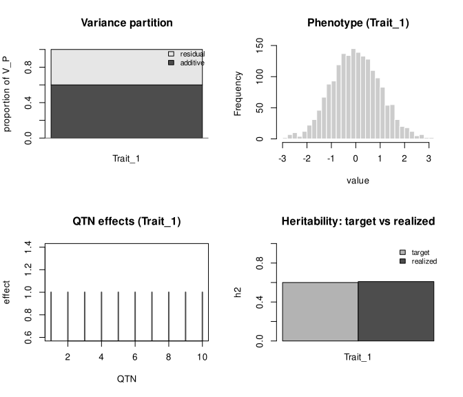
5.2 Assumptions and theory
5.2.1 The additive score
Write \(x_{ij}\) for the coded genotype of individual \(i\) at causal marker \(j\), with values -1, 0, 1, and \(b_j\) for the marker’s effect. The raw additive score is the weighted sum
\[ c_i = \sum_{j=1}^{m} x_{ij}\, b_j , \tag{5.1}\]
and the layer’s genetic value is the centered and rescaled score \(g_i = \sqrt{\pi}\,(c_i - \bar c)/s_c\), as derived in Section A.1. Here \(\pi\) is prop and \(s_c\) is the sample standard deviation of the scores. Both steps are package definitions, implemented in .component_raw() and .genetic_matrix(). The sample variance of \(g\) equals \(\pi\) exactly, whatever the effects and whatever the allele frequencies.
The coding counts one allele and is symmetric around the heterozygote; the model is linear in the number of copies, so it has no dominance. This is the v1 convention of the original publication (Fernandes and Lipka, 2020), not Fisher’s average-effect decomposition. For a single additive layer on a population in Hardy-Weinberg proportions the requested prop is the narrow-sense heritability of the simulated trait, because the whole genetic value is then additive.
5.2.2 Geometric effect series
The default effect of the \(k\)-th drawn marker is
\[ b_k = \beta^{\,k}, \qquad k = 1, \dots, m, \qquad \beta = 0.5 , \tag{5.2}\]
implemented in .effect_series(). The base \(\beta\) is the scalar effect; a base near one gives nearly equal effects and a small base concentrates the trait on the first few markers. With \(\beta = 0.5\) the tenth marker has an effect about a thousand times smaller than the first and is causal in name only. An explicit vector replaces the series. Because of the rescaling in the previous section, only ratios of effects matter.
Under phase = "repulsion" the series is multiplied by \((-1)^{k+1}\) in draw order. The package documents this as positional alternation, not a phase derived from linkage.
5.2.3 Why the variance explained depends on allele frequency
For a marker in Hardy-Weinberg proportions with allele frequency \(p\) of the counted allele, the variance of the -1, 0, 1 genotype code is \(2p(1-p)\). This is the variance of a binomial count with two trials, shifted by a constant. The variance of the marker’s contribution \(x_{ij} b_j\) is therefore \(2p(1-p)\,b_j^2\) in expectation. Two markers with the same effect can explain different shares of variance if their frequencies differ, and a rare allele with a large effect can explain less than a common allele with a smaller one.
In the maize panel every marker has a minor-allele frequency above 0.4, so \(2p(1-p)\) is close to its maximum of 0.5 and the ranking of var_explained follows the ranking of effects. In the mouse example the effects are equal, so the ranking follows \(2p(1-p)\) instead.
The package computes var_explained from the realized columns rather than from this expectation. Its definition (package convention, .qtn_var()) is the variance of the marker’s scaled column divided by the realized phenotypic variance, so it inherits the finite-sample frequencies and any departure from Hardy-Weinberg proportions. Inbred lines are an extreme departure: their genotype codes take almost only the values -1 and 1, and the code variance at frequency \(p\) is close to \(4p(1-p)\) rather than \(2p(1-p)\). The rescaling to prop absorbs this for the layer as a whole.
5.2.5 Seeds and reproducibility
With a non-missing seed, each layer draws its markers and effects under a sub-seed derived from the seed, the layer type, and the number of earlier layers of the same type (package scheme, .layer_seed()). Adding a dominance layer after an additive layer does not change the additive draw, which is why the chapters that follow can build on the simulations of this one. Inserting a second additive layer before an existing one does change the second one’s draw. The caller’s random-number state is left untouched.
5.3 Implementation and practical limits
The additive layer is pure R: marker sampling, effect generation, scaling, and residual draws all stay in R so that seeded results are reproducible across platforms. The internal functions named above are listed in the developer index.
n_qtnmust not exceed the number of markers that vary in the data. Monomorphic markers and markers heterozygous in every individual are never candidates.- A marker fixed with
qtnthat does not vary is accepted with a warning and contributes nothing. var_explainedis a diagnostic of one simulated sample. It is not an estimate and does not predict what an association study would detect.h2insimulate_phenotype()is the budget for additive, dominance, and epistatic layers together. With a single additive layer the layer may omitpropand take the whole budget.repsscales only the residual; the genetic value is unchanged. It does not model repeated measurements with a shared permanent environment.
TipChoosing the number of causal markers
A geometric series with base 0.5 makes the trait effectively oligogenic however large n_qtn is. For a polygenic trait raise the base toward one or give an explicit effect vector, and check the resulting var_explained column before trusting the architecture.