library(simplePHENOTYPES)
library(dplyr)
library(tibble)
library(readr)1 A first simulation
Suppose you have genotyped individuals and want to simulate a continuous trait controlled by 20 additive causal markers on their observed genotypes. You want to retain the simulated genetic values, inspect the phenotype, and save the result for a downstream analysis. This chapter carries out that workflow and checks what a requested genetic variance allocation of 0.5 actually means.
1.1 Worked example
1.1.1 Load the package
Use the development version corresponding to this book. The commands below assume the package is installed; see the build instructions if you are working from a source checkout.
1.1.2 Bring your own genotype data
The starting point is your genotype dataset. as_numeric() reads supported formats, including VCF and HapMap, and prepares the numeric input used by the simulation. Replace the path below with your own file. This recipe is not executed when building the book because it refers to a reader-supplied file.
geno <- as_numeric(
  "path/to/your_genotypes.vcf",
  to_r = TRUE, to_file = FALSE, verbose = FALSE
)
The same workflow accepts a HapMap file by replacing the path with, for example, "path/to/your_genotypes.hmp.txt". Format-specific dependencies and input checks are covered in the genotype input chapter. Before simulating, check individual identifiers, allele coding, missingness, and marker quality; importing a file does not establish that it is suitable for your study.
1.1.3 Follow along with observed maize genotypes
To make this chapter runnable without an external download, we use the bundled SNP55K_maize282_maf04 dataset: 10,650 markers and 280 maize individuals from an inbred association panel. The dataset name refers to the original 282-line panel; the bundled table contains 280 individual columns. Its documentation attributes the marker data to Cook et al. (2012); see ?SNP55K_maize282_maf04 for provenance.
These genotypes are already numeric. Here as_numeric() normalizes the input schema; it is not converting raw nucleotide calls. If you loaded your own file above, keep that geno object and skip this replacement block. All subsequent steps use the same object name.
data("SNP55K_maize282_maf04", package = "simplePHENOTYPES")
geno <- as_numeric(
  SNP55K_maize282_maf04,
  to_r = TRUE, to_file = FALSE, verbose = FALSE
)

tibble(markers = nrow(geno), individuals = ncol(geno) - 5)| markers | individuals |
|---|---|
| 10650 | 280 |
geno |>
  select(1:9) |>
head()| snp | allele | chr | pos | cm | 4226 | 4722 | 33-16 | 38-11 |
|---|---|---|---|---|---|---|---|---|
| ss196422159 | A/G | 1 | 379844 | 0.0000000 | -1 | -1 | -1 | -1 |
| ss196422171 | G/A | 1 | 613257 | 0.2482394 | -1 | -1 | -1 | -1 |
| ss196422173 | G/A | 1 | 659354 | 0.2972609 | 1 | 1 | -1 | -1 |
| ss196422186 | G/C | 1 | 992572 | 0.6515820 | 1 | -1 | -1 | -1 |
| ss196500940 | G/A | 1 | 2044264 | 1.7694445 | 1 | 1 | 1 | 1 |
| ss196422234 | A/G | 1 | 2044555 | 1.7697537 | -1 | -1 | -1 | -1 |
Markers occupy rows; the first five columns contain marker metadata and the remaining columns identify individuals. Genotypes use -1, 0, 1 coding; see coding conventions. The bundled data were filtered to minor allele frequency greater than 0.4 to reduce their size, so they do not represent the full allele-frequency spectrum of the original panel.
NoteObserved genotypes, simulated phenotype
The simulation uses the observed marker patterns, including their associations across loci, to generate a new trait. It does not use measured maize phenotypes. The bundled cm column is a synthetic genetic map, not measured recombination distances. This additive phenotype example does not simulate meiosis.
1.1.4 Specify and inspect the trait
sim <- simulate_phenotype(geno, seed = 901) |>
  additive(prop = 0.5, n_qtn = 20)
print(sim)
#> <phenotype_sim> (realized · long format)
#> Genotypes: geno Traits: 1 Architecture: independent Seed: 901
#> Variance partition (proportions of V_P):
#> additive 0.50 (20 QTNs, geometric)
#> residual 0.50
#> Requested genetic share = 0.50 realized H² = 0.48simulate_phenotype() establishes the simulation and its seed. additive() samples the causal markers and constructs the genetic component. The default effect series is geometric, so the 20 markers do not contribute equally. The object already contains realized phenotypes after the layer is added.
long <- phenotypes_long(sim)
wide <- phenotypes_wide(sim)
truth <- genetic_values(sim)
qt <- qtn_table(sim)

head(long)| id | trait | rep | value |
|---|---|---|---|
| 4226 | Trait_1 | 1 | 0.0612401 |
| 4722 | Trait_1 | 1 | -0.5645237 |
| 33-16 | Trait_1 | 1 | 0.1930537 |
| 38-11 | Trait_1 | 1 | 0.3056159 |
| A188 | Trait_1 | 1 | -1.1566117 |
| A239 | Trait_1 | 1 | -0.6677030 |
qt |>
  select(snp, effect, var_explained) |>
head()| snp | effect | var_explained |
|---|---|---|
| ss196468948 | 0.500000 | 0.3163513 |
| ss196448498 | 0.250000 | 0.0784679 |
| ss196439167 | 0.125000 | 0.0190034 |
| ss196524665 | 0.062500 | 0.0049463 |
| ss196489404 | 0.031250 | 0.0012104 |
| ss196434507 | 0.015625 | 0.0003081 |
The long table has one row per individual, trait, and simulation replication. The wide table has one trait column per trait. genetic_values() returns the simulated genetic values, and qtn_table() identifies the causal markers and their model effects. These are known simulation quantities, not estimates from phenotypes. The effect column is the layer’s effect series; component scaling also enters the realized genetic values, as explained below.
1.1.5 Check the realized variance
We compare what we requested with what the simulation produced. First, join phenotypes and genetic values by individual ID. as_tibble(..., rownames = "id") turns the genetic-value matrix into a table and keeps its individual names as an id column. left_join() matches individuals by that column, so row order does not matter.
In this example the phenotype is a genetic value plus a residual. Subtracting the genetic value therefore recovers the residual.
genetic <- truth |>
  as_tibble(rownames = "id") |>
  rename(genetic_value = Trait_1)

values <- long |>
  left_join(genetic, by = "id") |>
  mutate(residual = value - genetic_value)

comparison <- tibble(
  quantity = c(
    "Genetic variance", "Residual variance", "Genetic-residual covariance",
    "Phenotypic variance", "Genetic / phenotypic variance"
  ),
  parameter = c(0.5, 0.5, 0, 1, 0.5),
  simulated = c(
    var(values$genetic_value), var(values$residual),
    cov(values$genetic_value, values$residual), var(values$value),
    var(values$genetic_value) / var(values$value)
  )
)

comparison| quantity | parameter | simulated |
|---|---|---|
| Genetic variance | 0.5 | 0.5000000 |
| Residual variance | 0.5 | 0.5000000 |
| Genetic-residual covariance | 0.0 | 0.0233703 |
| Phenotypic variance | 1.0 | 1.0467406 |
| Genetic / phenotypic variance | 0.5 | 0.4776732 |
The parameter column shows the design values. The last two entries are the benchmarks obtained when genetic and residual components are uncorrelated; 0.5 is not a claim about the average of the sample variance ratio across runs. The genetic and residual sample variances equal 0.5 under the default settings. Their sample covariance can be positive or negative, so the last two rows can differ from their benchmarks. We explain why below.
plot(sim)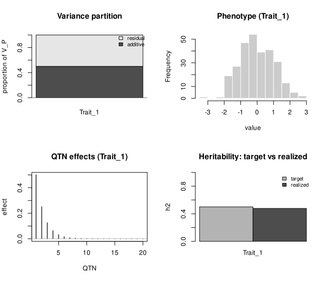
The default plot shows the variance budget, phenotype distribution, marker effects, and requested versus realized genetic variance ratio. The budget panel shows the model’s allocations; it is not a measurement of every sample variance. The histogram shows the resulting distribution; additive effects alone do not guarantee a bell-shaped phenotype distribution.
1.1.6 Export and reproduce the result
Create a results folder and save the phenotype and causal-marker tables. write_phenotypes() and write_qtn_table() use the simulation object directly.
dir.create("results", showWarnings = FALSE)
write_phenotypes(sim, file = "results/phenotypes.tsv", sep = "\t")
write_qtn_table(sim, file = "results/causal-markers.tsv", sep = "\t")

saved <- read_tsv("results/phenotypes.tsv", show_col_types = FALSE)
saved |> head()| id | trait | rep | value |
|---|---|---|---|
| 4226 | Trait_1 | 1 | 0.0612401 |
| 4722 | Trait_1 | 1 | -0.5645237 |
| 33-16 | Trait_1 | 1 | 0.1930537 |
| 38-11 | Trait_1 | 1 | 0.3056159 |
| A188 | Trait_1 | 1 | -1.1566117 |
| A239 | Trait_1 | 1 | -0.6677030 |
Use the same input and seed to repeat the simulation. The table below places the two sets of phenotypes next to each other.
again <- simulate_phenotype(geno, seed = 901) |>
  additive(prop = 0.5, n_qtn = 20)

first_run <- phenotypes_long(sim) |>
  rename(first_value = value)

second_run <- phenotypes_long(again) |>
  rename(second_value = value)

first_run |>
  left_join(second_run, by = c("id", "trait", "rep")) |>
  select(id, first_value, second_value) |>
head()| id | first_value | second_value |
|---|---|---|
| 4226 | 0.0612401 | 0.0612401 |
| 4722 | -0.5645237 | -0.5645237 |
| 33-16 | 0.1930537 | 0.1930537 |
| 38-11 | 0.3056159 | 0.3056159 |
| A188 | -1.1566117 | -1.1566117 |
| A239 | -0.6677030 | -0.6677030 |
The first rows illustrate reproducibility in this software environment. For a reproducible study, keep the input data, seed, and package version with your script.
1.2 Assumptions and theory
This example uses one continuous trait, one additive layer, one simulation replication, one record per individual, default mean zero, and a nondegenerate genetic component. There is no selection, crossing, dominance, epistasis, expression-mediated component, or threshold transformation.
1.2.1 How the trait is built
Each selected marker contributes its coded genotype multiplied by its effect. The package adds those contributions to obtain a genetic score for each individual. It then shifts the scores to mean zero and rescales them so their sample variance equals the requested allocation, here 0.5.
The residual represents variation outside this genetic component. By default, the package draws normal random values, shifts them to mean zero, and rescales them to the remaining variance, also 0.5. The phenotype is simply
\[ \text{phenotype} = \text{genetic value} + \text{residual}. \]
Rescaling controls the spread of each component. It does not control whether an individual with a high genetic value happens to receive a high residual too. The detailed normalization formulas are explained in Section A.1.
1.2.2 Why the realized ratio can differ from 0.5
Imagine two runs with exactly the same genetic values. In one run, individuals with high genetic values happen to receive mostly positive residuals. This reinforces their differences and increases the phenotype’s spread. In another run, those individuals happen to receive mostly negative residuals, reducing the spread. This chance agreement or disagreement is measured by sample covariance.
The exact accounting rule is
\[ \operatorname{Var}(y) = \operatorname{Var}(g) + \operatorname{Var}(e) + 2\operatorname{Cov}(g,e). \tag{1.1}\]
Here \(y\) means phenotype, \(g\) genetic value, and \(e\) residual. Var measures spread; Cov measures whether two sets of values tend to rise together. These are sample quantities, calculated from the simulated individuals.
Our two variances are 0.5 each. Their sum is one, but the covariance term can move phenotypic variance above or below one. Dividing genetic variance by this changing total therefore need not give exactly 0.5.
The package labels this sample ratio realized H². It is a diagnostic of one simulation, not an estimated population heritability. In unusual samples it can even exceed one; Section A.2 explains the algebra and gives an example. This does not imply that population heritability exceeds one.
1.2.3 Allow residual sample variance to fluctuate
Keep the default residual_mode = "fixed" when you want the residual component to have the same sample variance in each run. Choose "random" when you want ordinary normal sampling variation from independent normal residuals. In random mode, 0.5 describes the variance of the distribution supplying the residuals. A finite sample from that distribution need not have variance exactly 0.5, and its mean need not be exactly zero.
random_sim <- simulate_phenotype(geno, seed = 901, residual_mode = "random") |>
  additive(prop = 0.5, n_qtn = 20)

random_values <- phenotypes_long(random_sim) |>
  left_join(genetic, by = "id") |>
  mutate(residual = value - genetic_value)

tibble(
  quantity = c("Residual mean", "Residual variance", "Genetic-residual covariance"),
  parameter = c(0, 0.5, 0),
  fixed = c(
    mean(values$residual), var(values$residual),
    cov(values$genetic_value, values$residual)
  ),
  random = c(
    mean(random_values$residual), var(random_values$residual),
    cov(random_values$genetic_value, random_values$residual)
  )
)| quantity | parameter | fixed | random |
|---|---|---|---|
| Residual mean | 0.0 | 0.0000000 | 0.0477605 |
| Residual variance | 0.5 | 0.5000000 | 0.5062047 |
| Genetic-residual covariance | 0.0 | 0.0233703 | 0.0235149 |
The same seed and genetic specification retain the same genetic values, which is why we can reuse the genetic table. Random mode changes only how residuals are generated. Both modes leave genetic-residual sample covariance free to vary. For repeated sampling studies of estimators or confidence intervals, random mode matches a model with independent normal errors. Fixed mode offers controlled component variances for comparisons between simulation settings.
For multiple traits, resid_cor specifies their residual correlations. Random mode draws correlated normal residuals without fixing their sample variances. With reps, both modes divide residuals by the square root of the number of records to represent an entry mean. A carried population trait remembers its residual mode unless you explicitly choose another. For vQTLs, random mode also lets the heterogeneous residual component fluctuate; the average of its individual variance parameters equals the requested allocation.
1.2.4 Should the residual covariance be forced to zero?
Usually there is no need to force it to zero. Independent residual generation allows chance covariance in a finite sample; that is part of the sampling model. One could instead adjust the residuals using the genetic values until their sample covariance is zero, then rescale them. For this simple model that would make the variance ratio exactly 0.5, but it would impose another constraint on the sample. Such adjustment is a different simulation design and is not provided by either residual mode here.
1.2.5 How other simulators draw residuals
AlphaSimR’s ordinary setPheno() path, for example, draws independent normal residuals without fixing their sample variance or removing their chance covariance with the genetic values, which matches residual_mode = "random". Its h2 and H2 arguments calibrate the residual variance in the founder population, so the realized sample ratio still varies from population to population. The optional script dev/book/compare_alphasimr.R reproduces this comparison; other specialized model paths need separate interpretation.
1.3 Implementation and practical limits
The scientific calculations above are R functions. QTN sampling and effect and residual draws stay in R. The implementation diagram shows where Rust participates in other workflows.
- Preserve genotype orientation and individual identifiers when importing your own data.
- A requested positive allocation needs a component with nonzero variation.
- Interpret per-marker
var_explainedvalues as marginal contributions; covariance among marker contributions can prevent their sum from equaling the layer share. - This chapter’s residual calculation does not apply unchanged to threshold traits, expression-mediated phenotypes, or other added components.
TipExtending the maize example
This is an inbred panel. Before adding dominance, inspect heterozygosity: loci without heterozygotes cannot express variation in a heterozygote-indicator column. The high-MAF subset is a teaching dataset, not a universal marker-filtering rule.
1.3.1 Plant, animal, and human applications
The book’s worked examples use observed genotype datasets from all three contexts. Plant examples cover quantitative traits and breeding workflows on this maize panel; the prediction chapter uses heterogeneous-stock mice for relationships, prediction, and accuracy; and the binary phenotype chapter uses HapMap individuals to introduce liability_threshold(), distinguishing latent liability from observed case/control status. The genotype input chapter documents where each dataset comes from and how it is prepared.
The common starting point is a user’s genotype data. Dataset-specific features, such as inbreeding, relatedness, and population structure, belong in the scientific interpretation of each example.
1.4 Explore the simulation
Change the seed and compare the tables again. The component allocations should remain stable, while the sample covariance and realized ratio change. Then reduce the number of causal markers to one and inspect the phenotype histogram. Also repeat with residual_mode = "random" and watch the residual variance change. These comparisons distinguish model specification from the empirical distribution of one simulated population.