20 Inspecting and exporting results

A simulation is only useful once its phenotypes, genetic values, and causal markers reach the analysis that needs them. This chapter shows how to read a phenotype_sim object in R, how its tables are shaped when there are several traits and replications, what the diagnostic plot panels mean, and how to write the results as delimited text or JSON, including the marker data split into causal and non-causal files. It also checks that what is written can be read back unchanged.

20.1 Worked example

20.1.1 A two-trait, three-replication simulation

The maize example from the first chapter is extended to two traits and three simulation replications, with an additive layer and a dominance layer on the same loci. The inbred panel has very few heterozygotes, so a warning explains that dominance rests on fewer loci than requested; the dominance and epistasis chapter discusses that choice. Here the purpose is only to produce an object with enough structure to show every output shape.

library(simplePHENOTYPES)
library(dplyr)
library(tibble)
library(readr)

data("SNP55K_maize282_maf04", package = "simplePHENOTYPES")
geno <- as_numeric(
  SNP55K_maize282_maf04,
  to_r = TRUE, to_file = FALSE, verbose = FALSE
)

sim <- simulate_phenotype(geno, n_traits = 2, n_reps = 3, seed = 42) |>
  additive(prop = 0.4, n_qtn = 10) |>
  dominance(prop = 0.1, same_as_add = TRUE)

20.1.2 Read the printed summary

Printing the object is the first inspection. The method reports the genotype source, the number of traits, the architecture, the seed, and the variance partition that was requested for each layer, followed by the realized genetic-to-phenotypic variance ratio for each trait.

print(sim)

#> <phenotype_sim>  (realized · long format)
#>   Genotypes: geno   Traits: 2   Architecture: independent   Seed: 42
#>   Variance partition (proportions of V_P):
#>     additive    0.40   (10 QTNs, geometric)
#>     dominance   0.10   (same QTNs as additive)
#>     residual    [0.50, 0.50]
#>   Requested genetic share = [0.50, 0.50]   realized H² = [0.51, 0.51]
#>   Additive + dominance share loci (variance-partition coding); realized
#>   shares of V_P for the A+D block:
#>     Trait_1: requested 0.50 (unit-variance scale), realized 0.51
#>       = Var(A) 0.24 + Var(D) 0.16 + 2Cov(A,D) 0.12
#>       = Var(c_A) 0.42 + Var(c_D) 0.11 + 2Cov(c_A,c_D) -0.02
#>     Trait_2: requested 0.50 (unit-variance scale), realized 0.51
#>       = Var(A) 0.50 + Var(D) 0.12 + 2Cov(A,D) -0.11
#>       = Var(c_A) 0.41 + Var(c_D) 0.10 + 2Cov(c_A,c_D) -0.00
#>   ! realized - requested/V_P = (Var(c_A) + Var(c_D) - requested/V_P) +
#>     2Cov(c_A,c_D): the bracket is the covariance among same-type layers
#>     (0 for one additive and one dominance layer); the cross term depends
#>     on allele frequencies and on which allele is coded +1, and is not a
#>     finite-sample effect. For a Fisher-orthogonal additive/dominance split
#>     use additive(orthogonal = TRUE, a =, d =).

When additive and dominance layers share loci, the summary also decomposes the realized share into the two component variances and their covariance. That block is a diagnostic of this sample, in the sense explained in the first chapter: the requested proportions are what the layers were scaled to, and the realized values include the covariance between the additive and dominance components. As the printout says, that covariance is structural: it depends on allele frequencies and on which allele is coded +1, not on sampling noise.

20.1.3 Long and wide phenotype tables

phenotypes_long() returns one row per individual, trait, and replication. phenotypes_wide() returns one row per individual and replication, with one column per trait. Both are package definitions of the output layout, not transformations the reader has to perform.

long <- phenotypes_long(sim)
wide <- phenotypes_wide(sim)

tibble(
  layout = c("long", "wide"),
  rows = c(nrow(long), nrow(wide)),
  columns = c(ncol(long), ncol(wide))
)

layout	rows	columns
long	1680	4
wide	840	4

head(long)

id	trait	rep	value
4226	Trait_1	1	-0.5990545
4722	Trait_1	1	0.6675155
33-16	Trait_1	1	0.2499957
38-11	Trait_1	1	-0.0295282
A188	Trait_1	1	0.1612108
A239	Trait_1	1	1.3242920

head(wide)

id	rep	Trait_1	Trait_2
4226	1	-0.5990545	-0.1363557
4722	1	0.6675155	0.4705899
33-16	1	0.2499957	-1.2732480
38-11	1	-0.0295282	0.1458530
A188	1	0.1612108	0.8242908
A239	1	1.3242920	0.1194597

The long table has 280 individuals times 2 traits times 3 replications rows. The wide table collapses the trait dimension into columns, so it has half as many rows and the same four columns, with trait and value replaced by Trait_1 and Trait_2. Count rows per trait and replication to confirm that every combination is present once:

long |>
  count(trait, rep)

trait	rep	n
Trait_1	1	280
Trait_1	2	280
Trait_1	3	280
Trait_2	1	280
Trait_2	2	280
Trait_2	3	280

The long layout is what mixed-model software and plotting packages usually expect. The wide layout makes between-trait comparisons direct, for example a phenotypic correlation within a replication:

wide |>
  group_by(rep) |>
  summarise(phenotypic_correlation = cor(Trait_1, Trait_2))

rep	phenotypic_correlation
1	0.0940883
2	-0.0008183
3	0.1160749

20.1.4 Genetic values and the QTN table

genetic_values() returns an individuals-by-traits matrix of the genetic component before the residual was added. qtn_table() lists every causal marker with the effect it was given, one row per marker, trait, and layer.

truth <- genetic_values(sim)
head(truth)

#>          Trait_1    Trait_2
#> 4226  -0.8072176 -0.2955037
#> 4722  -0.1211446  0.6057121
#> 33-16 -0.2535059  0.2439101
#> 38-11 -0.2667421 -0.6660767
#> A188   0.7303801  0.3316197
#> A239   0.5980187 -0.6507275

qtn_table(sim) |>
  select(trait, layer, snp, chr, pos, maf, effect, var_explained) |>
  head()

trait	layer	snp	chr	pos	maf	effect	var_explained
Trait_1	additive	ss196434507	2	34417119	0.4803571	0.500000	0.3608476
Trait_1	additive	ss196434205	2	26263323	0.4857143	0.250000	0.0906017
Trait_1	additive	ss196435294	2	56929478	0.4785714	0.125000	0.0226273
Trait_1	additive	ss196480364	7	141719667	0.4089286	0.062500	0.0054590
Trait_1	additive	ss196474783	6	155105540	0.4285714	0.031250	0.0013879
Trait_1	additive	ss196469127	6	2045413	0.4571429	0.015625	0.0003516

The column meanings are package definitions:

Column	Meaning
`trait`, `layer`	The trait and the layer (`additive`, `dominance`, `epistasis`, `vqtl`, `transcriptome`) that uses the marker
`set`	For epistatic layers, the interacting set a marker belongs to; `NA` otherwise
`snp`, `chr`, `pos`	Marker identifier and map position copied from the genotype input; for a transcriptome layer `snp` holds a gene name
`maf`	Minor allele frequency in the simulated individuals
`effect`	The effect from the layer’s series (the additive effect `a` for an orthogonal layer)
`d`	The per-locus dominance deviation of an orthogonal layer; `NA` otherwise
`var_explained`	The marker’s marginal contribution to the trait variance
`QTN_t1`, `QTN_t2`, `ld_r2`	Always present; filled only under `architecture = "ld"` (the linked pair and its squared correlation) and `NA` otherwise

Both functions take a rep argument. In the simulation above, the replications share one genetic architecture, so rep makes no difference; only the residuals differ. With vary_qtn = TRUE each replication samples its own causal markers and effects, and rep selects which architecture to read:

vary <- simulate_phenotype(geno, n_reps = 3, vary_qtn = TRUE, seed = 7) |>
  additive(prop = 0.5, n_qtn = 4)

tibble(
  rep_1 = qtn_table(vary, rep = 1)$snp,
  rep_2 = qtn_table(vary, rep = 2)$snp,
  rep_3 = qtn_table(vary, rep = 3)$snp
)

rep_1	rep_2	rep_3
ss196414458	ss196439447	ss196514746
ss196468511	ss196508946	ss196513458
ss196513068	ss196476903	ss196492732
ss196455876	ss196499093	ss196477160

tibble(
  id = rownames(genetic_values(vary, rep = 1)),
  rep_1 = genetic_values(vary, rep = 1)[, 1],
  rep_2 = genetic_values(vary, rep = 2)[, 1]
) |>
  head()

id	rep_1	rep_2
4226	-0.8528983	0.6032541
4722	-0.6869417	-0.6763758
33-16	0.6407109	0.7632078
38-11	0.4747544	0.2833466
A188	-0.8528983	-0.1965146
A239	0.4747544	1.0831153

The three columns of marker names differ, and so do the genetic values of the same individual across replications. The default rep = 1 would silently describe only the first architecture; reading another replication’s phenotypes against the first replication’s QTN table would mismatch truth and data.

20.1.5 The diagnostic plot

plot() draws up to four panels. With two or more traits the fourth panel is the genetic-value scatter between the first two traits; with one trait it compares the requested and realized genetic share instead.

plot(sim)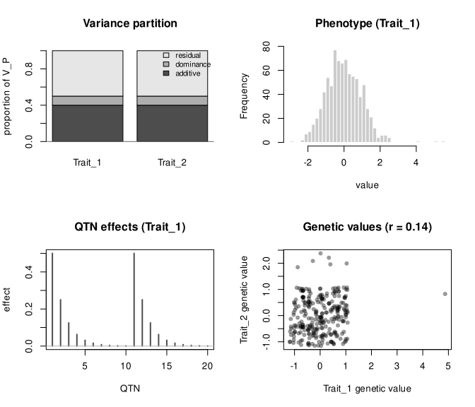

Diagnostic panels for the two-trait maize simulation: variance partition per trait, phenotype distribution of the first trait, effect sizes from the QTN table, and the genetic-value scatter between the two traits.

Panel	What it shows	What it does not show
`variance`	The requested proportion of each layer and the residual, stacked per trait	Realized sample variances or covariances between layers
`hist`	The realized phenotype distribution of the first trait, pooled over all replications	Other traits, or a single replication
`effects`	The `effect` column of `qtn_table()` for trait 1, replication 1	Other traits or replications, and variance explained, which also depends on allele frequency
`cor`	Genetic values of trait 1 against trait 2 when `n_traits > 1`; otherwise realized versus requested genetic share	Phenotypic correlation, which includes residual correlation

Select panels with which, for example plot(sim, which = "hist"), when a report needs a single figure.

20.1.6 Write phenotypes as text or JSON

write_phenotypes() writes the long table by default. The output directory must already exist. The format, separator, and file type are arguments; the examples below write three versions of the same phenotypes.

dir.create("results/export", showWarnings = FALSE, recursive = TRUE)

write_phenotypes(sim, file = "results/export/phenotypes.tsv")
write_phenotypes(sim, file = "results/export/phenotypes_wide.csv",
                 format = "wide", sep = ",")
write_phenotypes(sim, file = "results/export/phenotypes.json",
                 file_type = "json")

list.files("results/export")

#> [1] "phenotypes_wide.csv" "phenotypes.json"     "phenotypes.tsv"

Read them back to check the round trip. read_tsv() and read_csv() from readr parse the text files; jsonlite::read_json() with simplifyVector = TRUE turns the JSON array of row objects into a data frame.

from_tsv <- read_tsv("results/export/phenotypes.tsv", show_col_types = FALSE)
from_csv <- read_csv("results/export/phenotypes_wide.csv", show_col_types = FALSE)
from_json <- jsonlite::read_json("results/export/phenotypes.json",
                                 simplifyVector = TRUE)

tibble(
  file = c("phenotypes.tsv", "phenotypes_wide.csv", "phenotypes.json"),
  rows = c(nrow(from_tsv), nrow(from_csv), nrow(from_json)),
  max_abs_difference = c(
    max(abs(from_tsv$value - long$value)),
    max(abs(from_csv$Trait_1 - wide$Trait_1)),
    max(abs(from_json$value - long$value))
  )
)

file	rows	max_abs_difference
phenotypes.tsv	1680	0
phenotypes_wide.csv	840	0
phenotypes.json	1680	0

The text files are written with up to 15 significant digits, so values read back agree with the object to roughly machine precision rather than exactly. JSON values are written with 17 significant digits and read back exactly. Both statements are package definitions of the writers; the table shows the consequence for this simulation.

20.1.7 Write the QTN table

write_qtn_table() writes every column of qtn_table(). For a vary_qtn simulation, rep = "all" stacks the replications with a leading rep column so that the architectures stay distinguishable.

write_qtn_table(sim, file = "results/export/qtn_table.tsv")
write_qtn_table(vary, file = "results/export/qtn_table_all_reps.tsv",
                rep = "all")
write_qtn_table(sim, file = "results/export/qtn_table.json",
                file_type = "json")

read_tsv("results/export/qtn_table_all_reps.tsv", show_col_types = FALSE) |>
  select(rep, trait, layer, snp, effect, var_explained)

rep	trait	layer	snp	effect	var_explained
1	Trait_1	additive	ss196414458	0.5000	0.4638916
1	Trait_1	additive	ss196468511	0.2500	0.1165617
1	Trait_1	additive	ss196513068	0.1250	0.0289620
1	Trait_1	additive	ss196455876	0.0625	0.0072241
2	Trait_1	additive	ss196439447	0.5000	0.4382567
2	Trait_1	additive	ss196508946	0.2500	0.1106559
2	Trait_1	additive	ss196476903	0.1250	0.0277405
2	Trait_1	additive	ss196499093	0.0625	0.0069384
3	Trait_1	additive	ss196514746	0.5000	0.3053585
3	Trait_1	additive	ss196513458	0.2500	0.0769198
3	Trait_1	additive	ss196492732	0.1250	0.0189987
3	Trait_1	additive	ss196477160	0.0625	0.0048426

jsonlite::read_json("results/export/qtn_table.json", simplifyVector = TRUE) |>
  select(trait, layer, snp, effect) |>
  head(4)

trait	layer	snp	effect
Trait_1	additive	ss196434507	0.5000
Trait_1	additive	ss196434205	0.2500
Trait_1	additive	ss196435294	0.1250
Trait_1	additive	ss196480364	0.0625

20.1.8 Split the markers into causal and non-causal files

A downstream analysis often needs the genotypes without the causal markers, for example to study what a genome-wide association scan finds when the true loci are absent, with the truth kept separately. split_markers = TRUE writes the phenotype file together with three companions: the QTN table, the causal markers, and every non-causal marker. Default companion names are derived from file; markers_files overrides the two marker paths. The return value names every path written.

files <- write_phenotypes(vary, file = "results/export/vary.tsv",
                          split_markers = TRUE, rep = "all")
files

#>                                  phenotypes                                   qtn_table 
#>                   "results/export/vary.tsv"         "results/export/vary_qtn_table.tsv" 
#>                                      causal                                   noncausal 
#>       "results/export/vary_qtn_markers.tsv" "results/export/vary_noncausal_markers.tsv"

list.files("results/export", pattern = "^vary")

#> [1] "vary_noncausal_markers.tsv" "vary_qtn_markers.tsv"      
#> [3] "vary_qtn_table.tsv"         "vary.tsv"

The causal file uses the package’s numeric layout, five metadata columns and one column per individual, so it can be read back by as_numeric() or passed to simulate_phenotype() again. With rep = "all" the causal set is the union over replications: a marker causal in any selected replication is in the causal file and never in the non-causal file.

causal <- read_tsv(files[["causal"]], show_col_types = FALSE)
noncausal <- read_tsv(files[["noncausal"]], show_col_types = FALSE)

tibble(
  file = c("causal", "noncausal", "input"),
  markers = c(nrow(causal), nrow(noncausal), nrow(geno)),
  columns = c(ncol(causal), ncol(noncausal), ncol(geno))
)

file	markers	columns
causal	12	285
noncausal	10638	285
input	10650	285

causal |>
  select(snp, chr, pos, cm, 6:8)

snp	chr	pos	cm	4226	4722	33-16
ss196414458	1	41104295	42.19069	-1	-1	1
ss196514746	1	201489130	121.20797	1	1	-1
ss196513458	1	213090890	130.32121	1	1	1
ss196439447	2	161046323	94.47461	1	-1	1
ss196455876	4	127409885	80.58892	-1	1	1
ss196508946	5	20803111	21.94957	1	1	1
ss196468511	5	205375000	145.74105	-1	-1	-1
ss196476903	7	44690934	34.99405	-1	-1	-1
ss196477160	7	51472566	37.25698	1	-1	1
ss196513068	8	125183022	74.77590	1	1	1
ss196492732	9	107627382	62.65976	1	1	1
ss196499093	10	112573379	69.47247	-1	-1	1

The two marker counts add up to the number of input markers, and the causal markers are the union of the loci drawn in the three replications. The JSON layout differs: one object with individuals, markers, and, in the causal file, the qtn_table rows and a causal_for list on each marker that names the layers using it.

json_files <- write_phenotypes(
  sim, file = "results/export/split.json", file_type = "json",
  split_markers = TRUE,
  markers_files = c(causal = "results/export/causal_markers.json",
                    noncausal = "results/export/noncausal_markers.json")
)

causal_json <- jsonlite::read_json(json_files[["causal"]],
                                   simplifyVector = TRUE)
names(causal_json)

#> [1] "individuals" "qtn_table"   "markers"

length(causal_json$individuals)

#> [1] 280

causal_json$markers |>
  select(snp, chr, pos, maf) |>
  head(3)

snp	chr	pos	maf
ss196513147	1	88342158	0.4839286
ss196513825	1	174634851	0.4285714
ss196430291	1	217878023	0.4839286

causal_json$markers$causal_for[[1]]

trait	layer	set
Trait_1	additive	NA
Trait_1	dominance	NA

Each marker object carries its genotypes as an array in individuals order, and causal_for records that the first marker is used by both the additive and the dominance layer of the first trait.

20.2 Assumptions and theory

This chapter has no new statistical model. Its content is the set of package definitions that fix how simulation results are represented:

Table layouts. The long table is the canonical output, with columns id, trait, rep, and value. The wide table pivots trait into columns. Both come from the same realized values; neither is recomputed.
Genetic values. The matrix from genetic_values() is the sum of the scaled additive, dominance, and epistatic layers, and the genetically mediated part of a genome-derived transcriptome layer. A vqtl() layer modulates the residual spread and contributes no genetic value, so it is excluded. The complex architectures chapter returns to vQTLs.
Replications. n_reps requests simulation replications. Without vary_qtn, replications share the architecture and differ in their residual draws; with vary_qtn = TRUE they are independent architectures. The reps argument of the entry-mean model is a different quantity, as the conventions chapter explains.
Causal set. A marker is causal when any layer of any trait uses it in any selected replication. Gene rows of transcriptome layers are not markers and never appear in the marker files.

The var_explained column is a marginal quantity for each marker. Covariance among marker contributions, which arises from linkage disequilibrium in observed genotypes, means that the column need not sum to the layer’s proportion. The additive models chapter examines this.

20.3 Implementation and practical limits

Writers live in R; no compiled code is involved. Delimited text is written by data.table::fwrite(), JSON by jsonlite. Before writing companion files, the package checks that the directory exists and is writable, that no two paths resolve to the same file, and then moves the set into place as a group, so a failed write does not leave a partial set behind. These are package definitions documented in ?write_phenotypes.

Output directories must exist; write_phenotypes() does not create them.
Text output is not bit-for-bit; use JSON, or keep the R object, when exact values matter.
Default companion names are derived from file; passing a short file name keeps the companion names short as well.
The marker files use the genotypes of the simulated individuals. A phenotype built from expression alone has no markers, and split_markers = TRUE is an error in that case.
write_qtn_table() writes one replication by default. For a vary_qtn simulation pass rep = "all" so the file describes every replication of the phenotype file.
Specialized exporters of the frozen legacy interface, such as GEMMA .fam output, are not part of the grammar; the legacy chapter describes that interface.