library(simplePHENOTYPES)
library(dplyr)
library(tibble)

data("SNP55K_maize282_maf04", package = "simplePHENOTYPES")
geno <- as_numeric(
  SNP55K_maize282_maf04,
  to_r = TRUE, to_file = FALSE, verbose = FALSE
)

genetic_cor <- function(sim) cor(genetic_values(sim))7 Pleiotropy, linkage, and multiple traits
Two traits can be correlated because the same loci affect both (pleiotropy), because their distinct causal loci are inherited together (linkage), or because their non-genetic influences are shared (residual correlation). The package separates these mechanisms into three architectures and a residual correlation argument. This chapter simulates each one on the maize panel, compares requested with realized correlations, and explains which requests are attainable and why a realized correlation is a random quantity.
7.1 Worked example
The helper genetic_cor() is used throughout: it returns the sample correlation matrix of the simulated genetic values, the realized genetic correlation.
7.1.1 Independent traits
architecture = "independent" draws separate causal markers for each trait. prop may be a vector with one share per trait.
indep <- simulate_phenotype(geno, n_traits = 3, seed = 31) |>
  additive(prop = c(0.5, 0.3, 0.7), n_qtn = 20)
print(indep)
#> <phenotype_sim> (realized · long format)
#> Genotypes: geno Traits: 3 Architecture: independent Seed: 31
#> Variance partition (proportions of V_P):
#> additive [0.50, 0.30, 0.70] (20 QTNs, geometric)
#> residual [0.50, 0.70, 0.30]
#> Requested genetic share = [0.50, 0.30, 0.70] realized H² = [0.50, 0.28, 0.67]round(genetic_cor(indep), 3)#> Trait_1 Trait_2 Trait_3
#> Trait_1 1.000 -0.021 -0.179
#> Trait_2 -0.021 1.000 -0.175
#> Trait_3 -0.179 -0.175 1.000qtn_table(indep) |>
count(trait)| trait | n |
|---|---|
| Trait_1 | 20 |
| Trait_2 | 20 |
| Trait_3 | 20 |
The realized genetic correlations are not exactly zero. Different loci on the same genome still produce correlated values by chance, and in a panel with extensive linkage disequilibrium the chance correlations are not negligible. distinct_chr = TRUE puts each trait’s loci on different chromosomes, which removes within-chromosome linkage between traits but not chance correlation.
indep_chr <- simulate_phenotype(geno, n_traits = 3, seed = 31, distinct_chr = TRUE) |>
  additive(prop = 0.5, n_qtn = 20)

with(qtn_table(indep_chr), table(trait, chr))
#> chr
#> trait 1 10 2 3 4 5 6 7 8 9
#> Trait_1 8 1 0 0 6 0 0 5 0 0
#> Trait_2 0 0 8 0 0 4 0 0 8 0
#> Trait_3 0 0 0 12 0 0 5 0 0 3Each trait’s loci occupy a disjoint set of chromosomes.
7.1.2 Pleiotropy with a controlled genetic correlation
architecture = "pleiotropy" draws one set of loci shared by every trait and assigns each locus correlated effects across traits, so that the genetic correlation targets cor. The algorithm is PleioArch (Prado et al., in preparation), adopted as the package’s pleiotropy engine; the package prints a citation notice the first time cor is used in a session.
pleio <- simulate_phenotype(geno, n_traits = 2, architecture = "pleiotropy",
                            cor = 0.6, seed = 32) |>
  additive(prop = c(0.5, 0.3), n_qtn = 50)
print(pleio)
#> <phenotype_sim> (realized · long format)
#> Genotypes: geno Traits: 2 Architecture: pleiotropy Seed: 32
#> Variance partition (proportions of V_P):
#> additive [0.50, 0.30] (50 QTNs, geometric)
#> residual [0.50, 0.70]
#> Requested genetic share = [0.50, 0.30] realized H² = [0.57, 0.31]qtn_table(pleio) |>
select(trait, snp, effect, var_explained) |>
head(4)| trait | snp | effect | var_explained |
|---|---|---|---|
| Trait_1 | ss196515627 | -0.1971867 | 0.0163796 |
| Trait_1 | ss196511890 | 0.0645494 | 0.0017462 |
| Trait_1 | ss196496954 | -0.1529121 | 0.0098701 |
| Trait_1 | ss196469695 | -0.2770693 | 0.0321066 |
tibble(
  quantity = c("Genetic correlation", "Shared causal markers"),
  parameter = c(0.6, 50),
  simulated = c(genetic_cor(pleio)[1, 2], length(unique(qtn_table(pleio)$snp)))
)| quantity | parameter | simulated |
|---|---|---|
| Genetic correlation | 0.6 | 0.7187268 |
| Shared causal markers | 50.0 | 50.0000000 |
The effects are no longer a geometric series: they are drawn from a bivariate normal distribution whose covariance encodes the requested correlation, and each marker has one effect per trait. The realized correlation differs from 0.6, as the theory section explains.
7.1.3 Co-heritability
coheritability() standardizes the genetic covariance by the phenotypic standard deviations. Its diagonal is the realized broad-sense heritability of each trait and its off-diagonal is \(r_G h_1 h_2\), the quantity that predicts the correlated response of one trait to selection on the other in a purely additive model (Falconer and Mackay 1996, correlated response to selection).
coheritability(pleio)#> Trait_1 Trait_2
#> Trait_1 0.5697775 0.3034874
#> Trait_2 0.3034874 0.3129309h <- sqrt(diag(coheritability(pleio)))
tibble(
quantity = "Genetic correlation x h1 x h2",
from_coheritability = coheritability(pleio)[1, 2],
from_components = genetic_cor(pleio)[1, 2] * h[1] * h[2]
)| quantity | from_coheritability | from_components |
|---|---|---|
| Genetic correlation x h1 x h2 | 0.3034874 | 0.3034874 |
7.1.4 Partial pleiotropy
pi is the pleiotropic share of each trait’s genetic variance. With pi = 0.5, half of each trait’s additive variance comes from shared loci and half from loci specific to that trait. The shared loci appear in both traits’ rows of qtn_table(); the specific loci appear in one.
partial <- simulate_phenotype(geno, n_traits = 2, architecture = "pleiotropy",
                              cor = 0.4, pi = 0.5, seed = 32) |>
  additive(prop = 0.5, n_qtn = 50)

qtn_table(partial) |>
  count(snp, name = "traits_affected") |>
count(traits_affected, name = "markers")| traits_affected | markers |
|---|---|
| 1 | 50 |
| 2 | 25 |
tibble(
  quantity = "Genetic correlation",
  parameter = 0.4,
  simulated = genetic_cor(partial)[1, 2]
)| quantity | parameter | simulated |
|---|---|---|
| Genetic correlation | 0.4 | 0.3671036 |
Not every combination of cor and pi is possible. A correlation can only be as strong as the shared part of the variance allows; the package refuses an infeasible request instead of approximating it.
simulate_phenotype(geno, n_traits = 2, architecture = "pleiotropy",
                   cor = 0.8, pi = 0.5, seed = 32) |>
  additive(prop = 0.5, n_qtn = 50)
#> Error:
#> ! Biological constraint violated: cor^2 (0.64) cannot exceed pi_target * pi_secondary (0.25).7.1.5 A major pleiotropic locus
n_pleio_major and prop_var_major reserve a share of the shared variance for a few major loci. The first row of the table is the major locus.
major <- simulate_phenotype(geno, n_traits = 2, architecture = "pleiotropy",
                            cor = 0.6, n_pleio_major = 1, prop_var_major = 0.5,
                            seed = 32) |>
  additive(prop = 0.5, n_qtn = 50)

qtn_table(major) |>
  filter(trait == "Trait_1") |>
  select(snp, effect, var_explained) |>
head(3)| snp | effect | var_explained |
|---|---|---|
| ss196515627 | -0.8690521 | 0.3148948 |
| ss196511890 | -0.0784287 | 0.0025515 |
| ss196496954 | -0.1715781 | 0.0122995 |
7.1.6 Residual correlation
resid_cor sets the correlation of the residuals. The phenotypic correlation then mixes the genetic and residual correlations, weighted by the variance shares. The chunk recovers the residuals by subtracting genetic values from phenotypes and reports all three correlations.
mixed <- simulate_phenotype(geno, n_traits = 2, architecture = "pleiotropy",
                            cor = 0.6, resid_cor = -0.3, seed = 32) |>
  additive(prop = 0.5, n_qtn = 50)

wide <- phenotypes_wide(mixed)
g <- genetic_values(mixed)[wide$id, ]
e <- as.matrix(wide[, c("Trait_1", "Trait_2")]) - g

tibble(
  correlation = c("Genetic", "Residual", "Phenotypic"),
  parameter = c(0.6, -0.3, NA),
  simulated = c(cor(g)[1, 2], cor(e)[1, 2], cor(wide$Trait_1, wide$Trait_2))
)| correlation | parameter | simulated |
|---|---|---|
| Genetic | 0.6 | 0.7175986 |
| Residual | -0.3 | -0.3426565 |
| Phenotypic | NA | 0.1747257 |
Here the genetic and residual correlations have opposite signs and the phenotypic correlation sits between them. The theory section gives the weighting.
7.1.7 Correlations that decay with distance: repeated measurements
cor_ar1() builds a first-order autoregressive correlation matrix, \(R_{ij} = \rho^{|i-j|}\), for traits that are repeated measurements of one character over time or environments. Matrices are accepted both for cor and for resid_cor, and the one-call form sets everything at once.
cor_ar1(4, 0.8)#> Trait_1 Trait_2 Trait_3 Trait_4
#> Trait_1 1.000 0.80 0.64 0.512
#> Trait_2 0.800 1.00 0.80 0.640
#> Trait_3 0.640 0.80 1.00 0.800
#> Trait_4 0.512 0.64 0.80 1.000time_points <- simulate_phenotype(
geno, n_traits = 4, architecture = "pleiotropy",
cor = cor_ar1(4, 0.8), resid_cor = cor_ar1(4, 0.4),
h2 = 0.5, n_qtn = 40, seed = 33
)
round(genetic_cor(time_points), 2)#> Trait_1 Trait_2 Trait_3 Trait_4
#> Trait_1 1.00 0.85 0.65 0.29
#> Trait_2 0.85 1.00 0.83 0.53
#> Trait_3 0.65 0.83 1.00 0.75
#> Trait_4 0.29 0.53 0.75 1.00round(coheritability(time_points), 2)#> Trait_1 Trait_2 Trait_3 Trait_4
#> Trait_1 0.50 0.43 0.32 0.15
#> Trait_2 0.43 0.51 0.41 0.27
#> Trait_3 0.32 0.41 0.48 0.37
#> Trait_4 0.15 0.27 0.37 0.51Adjacent time points are more strongly correlated than distant ones, as requested, and the realized values scatter around the targets.
7.1.8 Linkage without pleiotropy
architecture = "ld" simulates two traits whose causal loci are distinct markers in linkage disequilibrium. For each locus of trait 1 the package finds a partner on the same chromosome whose squared correlation with it lies in the window [r2_min, r2_max], and that partner becomes a causal locus of trait 2. qtn_table() reports each pair and its squared correlation.
linked <- simulate_phenotype(geno, n_traits = 2, architecture = "ld",
                             r2_min = 0.4, r2_max = 0.9, seed = 34) |>
  additive(prop = 0.5, n_qtn = 10)
print(linked)
#> <phenotype_sim> (realized · long format)
#> Genotypes: geno Traits: 2 Architecture: ld Seed: 34
#> Variance partition (proportions of V_P):
#> additive 0.50 (10 QTNs, geometric)
#> residual [0.50, 0.50]
#> Requested genetic share = [0.50, 0.50] realized H² = [0.55, 0.52]qtn_table(linked) |>
filter(trait == "Trait_1") |>
select(QTN_t1, QTN_t2, chr, ld_r2) |>
head(5)| QTN_t1 | QTN_t2 | chr | ld_r2 |
|---|---|---|---|
| ss196463971 | ss196463973 | 5 | 0.8906343 |
| ss196507172 | ss196531126 | 4 | 0.7100644 |
| ss196445321 | ss196445319 | 3 | 0.7143284 |
| ss196445294 | ss196445308 | 3 | 0.8071321 |
| ss196458907 | ss196458918 | 4 | 0.7479153 |
No marker is causal for both traits, yet the genetic values are strongly correlated through linkage. Whether that correlation is positive or negative depends on which alleles travel together. ld_phase reads the sign of each pair’s dosage correlation and sets trait 2’s effect so that every pair pushes the correlation one way.
ld_phase_cor <- function(phase) {
  simulate_phenotype(geno, n_traits = 2, architecture = "ld",
                     r2_min = 0.4, r2_max = 0.9, ld_phase = phase, seed = 34) |>
    additive(prop = 0.5, n_qtn = 10) |>
    genetic_cor() |>
    (\(m) m[1, 2])()
}

tibble(
  ld_phase = c("coded", "coupling", "repulsion"),
  genetic_correlation = sapply(c("coded", "coupling", "repulsion"), ld_phase_cor)
)| ld_phase | genetic_correlation |
|---|---|
| coded | -0.8556967 |
| coupling | 0.9264180 |
| repulsion | -0.9264180 |
Under the default "coded" the sign follows the arbitrary marker coding; "coupling" makes it positive and "repulsion" negative, with the same loci and the same squared correlations.
7.1.9 How variable is a realized correlation?
The same request repeated with different seeds gives a spread of realized correlations. The spread is wider with few shared loci.
realized <- function(n_qtn, seeds = 1:20) {
  sapply(seeds, function(s) {
    simulate_phenotype(geno, n_traits = 2, architecture = "pleiotropy",
                       cor = 0.6, seed = s) |>
      additive(prop = 0.5, n_qtn = n_qtn) |>
      genetic_cor() |>
      (\(m) m[1, 2])()
  })
}

tibble(
  shared_loci = c(5, 50),
  parameter = 0.6,
  mean = c(mean(realized(5)), mean(realized(50))),
  sd = c(sd(realized(5)), sd(realized(50))),
  min = c(min(realized(5)), min(realized(50))),
  max = c(max(realized(5)), max(realized(50)))
)| shared_loci | parameter | mean | sd | min | max |
|---|---|---|---|---|---|
| 5 | 0.6 | 0.6577821 | 0.2009549 | 0.1636748 | 0.9314666 |
| 50 | 0.6 | 0.6308342 | 0.1209479 | 0.3947114 | 0.8237945 |
plot(pleio)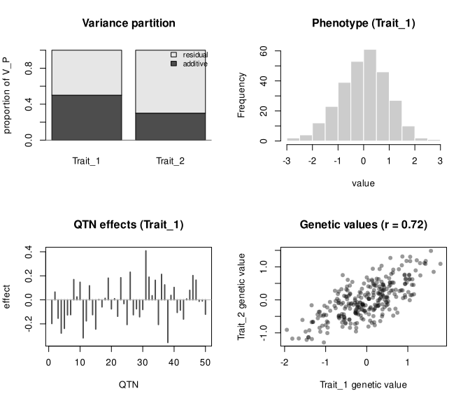
7.2 Assumptions and theory
7.2.1 The pleiotropic effect draw
Let \(V_t\) be trait \(t\)’s layer share (prop), \(\pi_t\) its pleiotropic share (pi, one by default), and \(r_{ts}\) the requested correlation. The shared loci receive effect vectors drawn from a multivariate normal distribution with covariance
\[ \Sigma_{tt} = \pi_t V_t, \qquad \Sigma_{ts} = r_{ts}\sqrt{V_t V_s}, \tag{7.1}\]
divided by the number of shared loci, and each trait-specific locus receives an independent normal effect with variance \((1-\pi_t)V_t\) divided by the number of specific loci (PleioArch, Prado et al., in preparation; the reference implementation is bundled with the package as simulateEffects.R, page not applicable; implemented in .pleio_draw()). Each effect is then divided by \(\sqrt{2\,\mathrm{MAF}(1-\mathrm{MAF})}\), the Hardy-Weinberg standard deviation of the genotype code, which converts an effect per standard deviation of the genotype code into an effect per allele.
With these moments, the expected genetic covariance between traits is \(r_{ts}\sqrt{V_t V_s}\) and each trait’s expected genetic variance is \(V_t\), so cor is the ratio of expected moments. The realized correlation is the ratio of sample moments and is therefore random. It converges to cor as the number of shared loci and the number of individuals grow, provided the causal loci are in approximate linkage equilibrium. With few shared loci it is attenuated toward zero on average; the package documentation reports an average of about 0.82 times cor with two shared loci. Strong linkage disequilibrium among the causal loci can prevent convergence altogether. These statements are package documentation backed by numerical checks, not literature results.
The layer rescaling of Section A.1 does not change a correlation, because it multiplies each trait’s values by a constant. It does fix each trait’s realized variance exactly at \(V_t\), so the only randomness left in the correlation is in the covariance.
7.2.2 Attainable requests
The covariance matrix in Equation 7.1 must be positive semi-definite. For two traits this reduces to
\[ r^2 \le \pi_1 \pi_2 , \tag{7.2}\]
which is the constraint printed by the error in the worked example. For more traits the package checks the matrix with diagonal \(\pi_t\) and off-diagonal \(r_{ts}\) by its smallest eigenvalue (algebraic generalization; the two-trait form follows the reference implementation). The rule has a plain reading: a correlation is carried only by the shared loci, so it cannot exceed what the shared variance can produce.
When the traits’ layer shares are not proportional across layers, for example mostly additive in one trait and mostly dominance in the other, the total genetic correlation falls short of cor; the package derives the large-sample target by covariance addition and warns when it differs from cor by more than one percent (package derivation, .pleio_total_cor_check()).
7.2.3 Phenotypic correlation from genetic and residual correlation
With genetic values \(g\) and residuals \(e\) for two traits and \(y = g + e\),
\[ \operatorname{Cov}(y_1, y_2) = \operatorname{Cov}(g_1, g_2) + \operatorname{Cov}(e_1, e_2) + \operatorname{Cov}(g_1, e_2) + \operatorname{Cov}(e_1, g_2). \tag{7.3}\]
In expectation the cross terms vanish, and dividing by the phenotypic standard deviations gives the familiar \(r_P = r_G h_1 h_2 + r_E \sqrt{(1-h_1^2)(1-h_2^2)}\). The simulated values are sample quantities, so the cross terms are not exactly zero and the realized phenotypic correlation deviates slightly from this formula. The first term is the off-diagonal element of coheritability().
In fixed residual mode, resid_cor mixes independently drawn residuals through the Cholesky factor of the requested matrix and re-standardizes each trait’s residual to its exact variance, so the residual variances are unchanged and only their correlation is induced. In random mode the residuals are a multivariate normal draw with the requested covariance as a parameter. A vqtl() component is drawn independently per trait and dilutes the residual correlation.
7.2.4 Linkage disequilibrium between distinct loci
Under "ld" the squared correlation between two markers’ genotype codes is the package’s measure of linkage disequilibrium, the genotypic or composite \(r^2\) (standard Pearson correlation on dosages; page unverified). The default partner = "strongest" takes the in-window partner with the highest \(r^2\), so the realized values skew toward r2_max; partner = "random" draws uniformly within the window. The resulting genetic correlation is a sum over pairs of \(b_1 b_2\, r\), where \(r\) is the signed dosage correlation and \(b_1\), \(b_2\) are the pair’s effects, plus cross-pair terms between loci of different pairs that happen to be in LD. ld_phase controls the sign pair by pair but not the cross-pair terms, so on a chromosome with many nearby pairs the total can still differ in sign from the pairs’ common sign. The "ld" design follows DECISION-014 of the project decision log; the linkage concept comes from the original publication, with the v2 algorithm being a package design.
7.3 Implementation and practical limits
The effect draws stay in R and are seeded per layer. The PleioArch draw uses a symmetric eigenvalue square root of the covariance matrix rather than the reference implementation’s Cholesky factor, which gives the same distribution but different realizations, and allows exactly singular feasible requests.
"ld"requiresn_traits = 2, one additive layer, and at most a dominance layer on the same linked loci. Epistasis and user-fixed loci are rejected under"ld"with random pairs;qtn = list(trait1, trait2)is accepted for direct pairs.- Under
"pleiotropy", user-suppliedeffectis accepted only when no correlation is controlled;qtnfixes the shared loci butpi < 1cannot then be used. - A single shared locus makes the realized correlation plus or minus one; the package warns.
- The realized correlation on a fixed sample of individuals cannot beat the sampling spread of a correlation over that many individuals, however many loci are shared.
- Most of the scatter of the realized correlation around its target comes from drawing a finite number of effect pairs, with a standard deviation of about \((1-r^2)/\sqrt{n_{qtn}-1}\). Linkage disequilibrium in the maize panel adds to it.
NotePartial pleiotropy by trait-specific layers
pi splits one layer into shared and specific loci. For loci that affect only some traits with layer-specific settings, or to combine several simulations into one trait, see complex_phenotypes() in the complex architectures chapter.