library(simplePHENOTYPES)
library(dplyr)
library(tibble)4 Maps, haplotypes, and founders
Suppose you want to simulate crosses, selfing, or doubled haploids from your genotyped individuals. A dosage table is not enough: meiosis needs to know which allele sits on which of the two homologous chromosomes and how far apart markers are in recombination units. This chapter builds a Population from real genotypes, inspects its haplotypes, supplies a genetic map when the data have none, and generates founders from a coalescent model when you have no genotypes at all.
4.1 Worked example
4.1.1 Load the packages
4.1.2 Founders from the maize panel
The bundled maize data carry a cm column, so as_population() can use them directly. The print method summarizes the individuals, markers, genetic map, and pedigree status.
data("SNP55K_maize282_maf04", package = "simplePHENOTYPES")
maize <- as_numeric(SNP55K_maize282_maf04, to_r = TRUE, to_file = FALSE,
                    verbose = FALSE)

founders <- as_population(maize)
founders
#> <Population>
#> Individuals: 280 Markers: 10650 Chromosomes: 10
#> Genetic map: 1497 cM total span (109-219 cM per chromosome)
#> Origin: founder
#> Pedigree: 280 recorded individuals; generation 0
#> IDs: 4226, 4722, 33-16, 38-11, A188, A239, ... (274 more)n_individuals(founders)#> [1] 280Every individual is recorded as a pedigree founder in generation 0. The population keeps the marker map and a pedigree table; both are plain data frames you can inspect.
founders$map |> head(3)| snp | chr | pos | cm | allele |
|---|---|---|---|---|
| ss196422159 | 1 | 379844 | 0.0000000 | A/G |
| ss196422171 | 1 | 613257 | 0.2482394 | G/A |
| ss196422173 | 1 | 659354 | 0.2972609 | G/A |
founders$pedigree |> select(id, mother, father, generation, design) |> head(3)| id | mother | father | generation | design |
|---|---|---|---|---|
| 4226 | NA | NA | 0 | founder |
| 4722 | NA | NA | 0 | founder |
| 33-16 | NA | NA | 0 | founder |
4.1.3 Dosages and haplotypes
dosages() returns the markers-by-individuals -1/0/1 matrix. haplotypes() returns the two strands, called cis and trans, with 1 marking the counted allele. The dosage is the sum of the two strands minus one, and we check that identity on the whole panel.
d <- dosages(founders)
h <- haplotypes(founders)

d[1:3, 1:4]
#> 4226 4722 33-16 38-11
#> ss196422159 -1 -1 -1 -1
#> ss196422171 -1 -1 -1 -1
#> ss196422173 1 1 -1 -1h$cis[1:3, 1:4]#> 4226 4722 33-16 38-11
#> ss196422159 0 0 0 0
#> ss196422171 0 0 0 0
#> ss196422173 1 1 0 0tibble(
quantity = c("markers", "individuals", "dosage equals cis + trans - 1"),
value = c(nrow(d), ncol(d), identical(h$cis + h$trans - 1L, d))
)| quantity | value |
|---|---|
| markers | 10650 |
| individuals | 280 |
| dosage equals cis + trans - 1 | 1 |
The strands have no parental meaning. Meiosis treats them symmetrically, so either assignment is valid as long as both strands of an individual stay together.
4.1.4 Selecting individuals
Subsetting with [ keeps the selected individuals in the order given, by name, position, or logical mask. A repeated subscript duplicates an individual: the copy receives a unique id but shares the original’s pedigree key, so the pedigree still records one individual.
parents <- founders[c("33-16", "38-11")]
parents
#> <Population>
#> Individuals: 2 Markers: 10650 Chromosomes: 10
#> Genetic map: 1497 cM total span (109-219 cM per chromosome)
#> Origin: founder
#> Pedigree: 2 recorded individuals; generation 0
#> IDs: 33-16, 38-11twice <- founders[c(1, 1, 2)]
twice$ids#> [1] "4226" "4226_1" "4722"nrow(twice$pedigree)#> [1] 2as_population() accepts the same selection through its individuals argument, which avoids phasing the full panel when only a few lines are needed.
4.1.5 Outbred founders and the phasing guess
The maize lines are almost completely homozygous, so their haplotypes are nearly determined by the dosages. The human panel is different. We load it with the helper described in Genotype input and quality control, give it a synthetic map, and phase the first 50 individuals.
source("_data.R")
human <- book_human()
human$cm <- synthetic_map(human$chr, human$pos, cm_per_mb = 1)

people <- as_population(human, individuals = 1:50)
people
#> <Population>
#> Individuals: 50 Markers: 9028 Chromosomes: 23
#> Genetic map: 2905 cM total span (31-245 cM per chromosome)
#> Origin: founder
#> Pedigree: 50 recorded individuals; generation 0
#> IDs: NA19152, NA19139, NA18912, NA19160, NA07034, NA07055, ... (44 more)strands <- haplotypes(people)
het <- dosages(people) == 0
tibble(
heterozygous_calls = sum(het),
cis_carries_counted_allele = sum(strands$cis[het] == 1),
trans_carries_counted_allele = sum(strands$trans[het] == 1)
)| heterozygous_calls | cis_carries_counted_allele | trans_carries_counted_allele |
|---|---|---|
| 120292 | 120292 | 0 |
Every heterozygote has been placed with the counted allele on the first strand. That is a rule, not an inference: the dosage table does not say which allele sits on which chromosome, and the package does not import external phase. For these founders, all heterozygous sites on a chromosome are in perfect coupling, so their first-generation gametes carry more linkage disequilibrium than real gametes would. The founders’ own dosages are exact, but every gamete they produce, from the first cross on, carries this coupling-phase linkage disequilibrium. Use population_from_haplotypes() with phased data whenever meiosis of outbred founders matters.
4.1.6 Founders from known haplotypes
When the phase is known, from statistically phased data or another simulator, population_from_haplotypes() builds the population from the two strand matrices directly. Here we rebuild the human founders from their own strands and confirm that the dosages agree, then construct a two-individual example by hand where one individual is heterozygous at two linked markers with a specified phase.
rebuilt <- population_from_haplotypes(strands$cis, strands$trans, people$map,
                                      pool = "hapmap")
identical(dosages(rebuilt), dosages(people))
#> [1] TRUEmap <- data.frame(snp = paste0("m", 1:4), chr = 1, pos = c(100, 200, 300, 400),
cm = c(0, 10, 20, 30))
cis <- cbind(ind1 = c(1, 1, 0, 0), ind2 = c(0, 0, 0, 0))
trans <- cbind(ind1 = c(1, 0, 1, 0), ind2 = c(0, 0, 0, 0))
known <- population_from_haplotypes(cis, trans, map)
dosages(known)#> ind1 ind2
#> m1 1 -1
#> m2 0 -1
#> m3 0 -1
#> m4 -1 -1haplotypes(known)$cis#> ind1 ind2
#> m1 1 0
#> m2 1 0
#> m3 0 0
#> m4 0 0Individual ind1 is heterozygous at m2 and m3, with the counted allele at m2 on the first strand and at m3 on the second: repulsion phase. as_population() would have put both on the first strand. The meiosis chapter shows how that difference changes the gametes.
4.1.7 A map for data without one
The mouse genotypes carry physical positions but no genetic map, so as_population() refuses them until cm is filled. synthetic_map() converts base pairs into a plausible centiMorgan map. It starts each chromosome at 0 and is non-decreasing within a chromosome.
mice <- book_mice()
mice$cm <- synthetic_map(mice$chr, mice$pos)

tibble(chr = mice$chr, pos = mice$pos, cm = mice$cm) |>
  group_by(chr) |>
  summarise(markers = n(), span_mb = max(pos) / 1e6,
            length_cm = max(cm), .groups = "drop") |>
head(5)| chr | markers | span_mb | length_cm |
|---|---|---|---|
| 1 | 875 | 118.12702 | 86.23272 |
| 10 | 334 | 83.38167 | 60.86862 |
| 11 | 647 | 93.48675 | 68.24533 |
| 12 | 490 | 69.33921 | 50.56961 |
| 13 | 415 | 69.57477 | 50.78958 |
mouse_founders <- as_population(mice, individuals = 1:100)
mouse_founders
#> <Population>
#> Individuals: 100 Markers: 10346 Chromosomes: 20
#> Genetic map: 1180 cM total span (39-86 cM per chromosome)
#> Origin: founder
#> Pedigree: 100 recorded individuals; generation 0
#> IDs: A048005080, A048006063, A048006555, A048007096, A048010273, A048010371, ... (94 more)
NoteThis map is a model
The cm values are not estimates of mouse recombination distances. They give the simulation a recombination landscape with the right order of magnitude and centromeric suppression. If you have a measured map for your markers, put it in cm instead.
The default rate of 0.73 cM per Mb is a maize-scale value. The shape of the map comes from a local rate that dips around the centromere, which defaults to the midpoint of each chromosome’s span. Setting suppression = 0 gives a uniform map, and total_cm fixes chromosome lengths directly.
on1 <- mice$chr == "1"
uniform <- synthetic_map(mice$chr, mice$pos, suppression = 0)
plot(mice$pos[on1] / 1e6, mice$cm[on1], type = "l", lwd = 2,
     xlab = "Physical position on chromosome 1 (Mb)",
     ylab = "Genetic position (cM)")
lines(mice$pos[on1] / 1e6, uniform[on1], lwd = 2, lty = 2, col = "grey50")
legend("topleft", c("centromere-suppressed", "uniform"),
       lwd = 2, lty = c(1, 2), col = c("black", "grey50"), bty = "n")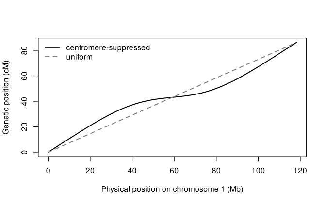
fixed <- synthetic_map(mice$chr, mice$pos, total_cm = 80)
tibble(chr = mice$chr, default = mice$cm, uniform = uniform, fixed = fixed) |>
  group_by(chr) |>
  summarise(across(c(default, uniform, fixed), max), .groups = "drop") |>
head(4)| chr | default | uniform | fixed |
|---|---|---|---|
| 1 | 86.23272 | 86.23272 | 80 |
| 10 | 60.86862 | 60.86862 | 80 |
| 11 | 68.24533 | 68.24533 | 80 |
| 12 | 50.56961 | 50.56961 | 80 |
4.1.8 Founders without genotypes
founders_coalescent() simulates founder haplotypes under a sequential Markov coalescent with recombination and mutation, using the same demographic presets that AlphaSimR’s runMacs() builds. The result is a Population whose counted allele is the derived allele. The seed makes it reproducible.
generic <- founders_coalescent(50, n_chr = 2, seg_sites = 500, seed = 1)
generic
#> <Population>
#> Individuals: 50 Markers: 1000 Chromosomes: 2
#> Genetic map: 199 cM total span (99-100 cM per chromosome)
#> Origin: founder
#> Pedigree: 50 recorded individuals; generation 0
#> IDs: 1, 2, 3, 4, 5, 6, ... (44 more)again <- founders_coalescent(50, n_chr = 2, seg_sites = 500, seed = 1)
identical(dosages(again), dosages(generic))#> [1] TRUEattr(generic, "coalescent")$n_total#> [1] 20954 20065seg_sites keeps a uniform random subset of the segregating sites the coalescent produced; the attribute records how many existed before subsetting. A constant-size neutral coalescent sample has a spectrum skewed toward rare variants. The "GENERIC" preset instead follows AlphaSimR’s demography, a recent strong bottleneck, which depletes rare variants, so the median minor allele frequency in the summary is well above what a constant-size sample would give.
x <- dosages(generic)
p <- rowMeans(x + 1) / 2
tibble(
  quantity = c("minimum MAF", "median MAF", "fraction heterozygous"),
  value = c(min(pmin(p, 1 - p)), median(pmin(p, 1 - p)), mean(x == 0))
)| quantity | value |
|---|---|
| minimum MAF | 0.01000 |
| median MAF | 0.22000 |
| fraction heterozygous | 0.31564 |
Species presets change the chromosome length, mutation and recombination parameters, and the population-size history. inbred = TRUE duplicates each simulated haplotype so every founder is homozygous, the usual starting point for a line-breeding program. split separates the founders into two subpopulations with no migration for a number of generations before the present.
maize_like <- founders_coalescent(50, n_chr = 2, seg_sites = 500,
                                  species = "MAIZE", seed = 1)
maize_like
#> <Population>
#> Individuals: 50 Markers: 1000 Chromosomes: 2
#> Genetic map: 397 cM total span (198-199 cM per chromosome)
#> Origin: founder
#> Pedigree: 50 recorded individuals; generation 0
#> IDs: 1, 2, 3, 4, 5, 6, ... (44 more)lines <- founders_coalescent(20, seg_sites = 300, inbred = TRUE, seed = 2)
all(dosages(lines) != 0)#> [1] TRUEsplit_pop <- founders_coalescent(40, seg_sites = 300, split = 50, seed = 3)
xs <- dosages(split_pop)
p1 <- rowMeans(xs[, 1:20] + 1) / 2
p2 <- rowMeans(xs[, 21:40] + 1) / 2
tibble(mean_absolute_frequency_difference = mean(abs(p1 - p2)))| mean_absolute_frequency_difference |
|---|
| 0.1920833 |
The last table is a descriptive statistic of the two halves’ allele frequencies, not an estimator of a population parameter.
4.2 Assumptions and theory
4.2.1 Phasing and dosage rules
For an individual’s dosage \(x_j \in \{-1, 0, 1\}\) at marker \(j\), as_population() sets
\[ \text{cis}_j = \mathbf{1}[x_j \ge 0], \qquad \text{trans}_j = \mathbf{1}[x_j > 0], \tag{4.1}\]
so homozygotes are determined and every heterozygote has its counted allele on the first strand. This is a package convention; the equation map records it for as_population(). The inverse,
\[ x_j = \text{cis}_j + \text{trans}_j - 1, \tag{4.2}\]
is the isqg genotype_num convention that dosages() and the Rust genome module implement. The identity check above executes it.
4.2.2 The synthetic map model
synthetic_map() assigns each physical position \(p\) on a chromosome of span \(L\) a local rate
\[ r(p) = 1 - s \exp\!\left(-\tfrac{1}{2}\left(\frac{p - c}{wL}\right)^2\right), \tag{4.3}\]
where \(c\) is the centromere position, \(s\) the suppression strength and \(w\) the relative width of the suppressed region. The rate is integrated across marker intervals and rescaled so that the chromosome reaches its target length, either total_cm or cm_per_mb times the span in Mb. Because \(r(p)\) is positive for \(s < 1\), cM is a monotone function of bp.
The Gaussian form is a phenomenological package choice. The package documentation cites Bauer et al. (2013) for the pericentromeric suppression pattern in maize and the genome-wide scale the defaults approximate, and states that the functional form and parameters are not taken from that source. The map’s length matters for what follows: the expected number of crossovers on a chromosome equals its last map position in Morgans, as the meiosis chapter explains.
4.2.3 The coalescent founders
founders_coalescent() follows the model documented for the function: time in units of \(4N_0\) generations, per-chromosome \(\theta = 4N_0\mu\) and \(\rho = 4N_0 r\), a piecewise-constant population-size history relative to \(N_0\), infinite-sites mutation, and a sequential Markov coalescent (SMC’) walk along the chromosome. The genetic map is linear in physical position and starts at 0 cM at the first segregating site. The species presets reproduce the demographic commands that AlphaSimR 2.1.0’s runMacs() builds; their parameter values are AlphaSimR’s choices, not estimates made in this package. The package references are Marjoram and Wall (2006), Chen, Marjoram and Wall (2009), Hudson (2002), and Gaynor, Gorjanc and Hickey (2021), as given in the function documentation. This book does not verify the coalescent algorithm against those sources; the allele-frequency summary above is a sanity check of the output, not a validation of the model.
4.2.4 Randomness and reproducibility
This function is the one place where random numbers are drawn in Rust. Its pseudorandom generator is seeded from R, so a seed reproduces the founders and the caller’s R random state is restored afterwards. Meiosis, QTN sampling, and effect and residual draws remain in R, as described in the implementation overview.
4.3 Implementation and practical limits
as_population() and population_from_haplotypes() are R functions in the crossing module; dosages() combines the strands through the Rust genome code; founders_coalescent() calls coalescent_chromosome_core() per chromosome and assembles the result with population_from_haplotypes(). The developer index gives current locations.
cmmust be in centiMorgans, non-decreasing within a chromosome, with no missing values; a map whose largest value is at most 5 across 20 or more markers draws a warning because it looks like Morgans.- Chromosomes are processed in a canonical order (numeric labels first), so
chrstored as text or as numbers gives the same seeded progeny. - Populations built from separately converted panels can count different alleles as
1. Convert jointly or carry thecountedcolumn, as the input chapter describes;cross()andc.Population()stop when the records disagree. - Phasing a large outbred panel is fast, but the phase is a guess. Use
population_from_haplotypes()when real phase information exists. founders_coalescent()can return fewer segregating sites than requested only by stopping with an error; ask for fewer sites or more individuals.- A filtered population (see
filter_geno()) has a different marker set from the unfiltered one and cannot be crossed or pooled with it.